

Risk-adjusted returns measure how much return an investment delivers per unit of risk taken. That single idea separates serious performance analysis from raw-return scorekeeping. The Sharpe ratio is the default starting metric for most practitioners, U.S. Treasury yields serve as the standard risk-free benchmark, and tools like Strategyprofilers let algorithmic traders compute these measures across combined portfolios rather than strategy by strategy.
- Verdict: A higher return means nothing if it came with twice the risk. Risk-adjusted metrics normalize performance so you can compare a bond fund to an equity strategy on equal footing.
- Quick action: Start with the Sharpe ratio. If your strategy has a skewed payoff or heavy drawdowns, follow up with the Sortino and Calmar ratios.
- Caution: No single ratio tells the full story. Relying on Sharpe alone can mask drawdown risk, volatility clustering, and overfitting in backtests.
Pro Tip: When your strategy has a holding period under one year, use the 3-month U.S. Treasury bill yield as the risk-free rate. For long-horizon strategies, the 10-year Treasury yield is more appropriate.
Table of Contents
- What are risk-adjusted returns and why do they matter?
- The main risk-adjusted metrics: formulas and inputs
- How to calculate Sharpe and Sortino: a worked example
- How to interpret ratio values and set benchmarks
- Which risk-adjusted metric should you use?
- Where risk-adjusted metrics can mislead you
- How to apply these metrics in portfolio construction
- Applying risk-adjusted metrics to algorithmic trading portfolios
- Key Takeaways
- The metrics are only as honest as the process behind them
- Strategyprofilers puts these metrics to work for algorithmic traders
- Useful sources and further reading
What are risk-adjusted returns and why do they matter?
A raw return tells you what happened. A risk-adjusted return tells you whether it was worth the risk to get there. Two funds both returning 12% annually look identical until you see that one achieved it with 8% annualized volatility and the other with 22%. The first is a fundamentally different investment.
The mechanics rely on a risk-free benchmark, typically U.S. Treasury yields, which represent the return you could earn without taking on market risk. Any return above that threshold is the "excess return" you earned by accepting risk. Dividing that excess return by a measure of risk produces a ratio that lets you compare strategies across asset classes, time horizons, and management styles.
Practitioners use these metrics in three main contexts:
- Performance evaluation: Determining whether a manager or strategy added value relative to the risk taken, not just relative to a benchmark.
- Manager selection: Screening candidates by minimum ratio thresholds during due diligence. Institutional allocators commonly set floors on Sharpe and Calmar ratios before a strategy qualifies for allocation.
- Portfolio construction: Allocating capital toward strategies with the highest risk-adjusted contribution, not the highest raw return.
The CFA Institute treats risk-adjusted measures as central to GIPS-consistent performance reporting, precisely because raw returns conflate luck and risk-taking with genuine skill. A manager who ran concentrated positions in a bull market looks brilliant on raw returns. Adjust for the risk they took, and the picture often changes.
BlackRock frames the concept as a behavioral discipline: treating risk-adjusted performance as a "speed limit" reduces the temptation to chase short-term trends that increase accident risk. That framing is useful. The metrics are not just math. They are a check on the instinct to reach for return without accounting for what you are risking to get it.
Pro Tip: For strategies benchmarked against equity indices, use the 10-year Treasury yield as the risk-free rate. For cash-like or short-duration strategies, the 3-month T-bill rate is more appropriate and avoids overstating excess return.
The main risk-adjusted metrics: formulas and inputs
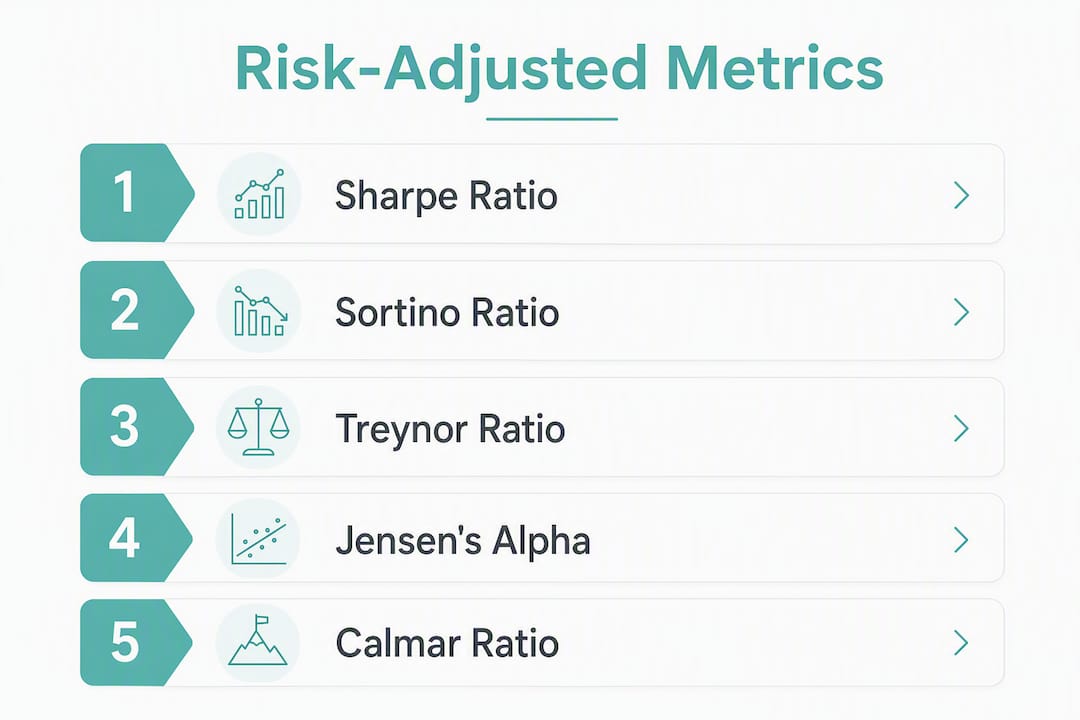
Every metric below answers a slightly different question about the risk return tradeoff. Knowing which question each one asks is as important as knowing the formula.

Sharpe ratio
Formula: (Rp − Rf) ÷ σp
- Rp = portfolio return (annualized)
- Rf = risk-free rate (annualized U.S. Treasury yield)
- σp = annualized standard deviation of portfolio returns
Annualizing from monthly returns: multiply monthly return by 12, multiply monthly standard deviation by √12. From daily returns, multiply by 252 trading days and √252 respectively.
Sortino ratio
Formula: (Rp − T) ÷ Downside Deviation
- T = target or minimum acceptable return (often the risk-free rate)
- Downside Deviation = standard deviation of returns below T only
The Sortino ratio penalizes only negative volatility, making it more appropriate for strategies with positively skewed return distributions.
Treynor ratio
Formula: (Rp − Rf) ÷ βp
- βp = portfolio beta relative to a market benchmark
Treynor measures excess return per unit of systematic risk. Use it when the portfolio is one sleeve inside a larger, diversified allocation.
Jensen's alpha
Formula: α = Rp − [Rf + βp × (Rm − Rf)]
- Rm = benchmark or market return
- α = return above or below what CAPM predicts given the portfolio's beta
A positive alpha indicates the manager added return beyond what market exposure alone would explain. The CFA Institute specifically highlights Jensen's alpha as a tool for isolating manager skill from market exposure.
Information ratio
Formula: (Rp − Rb) ÷ Tracking Error
- Rb = benchmark return
- Tracking Error = standard deviation of (Rp − Rb)
The information ratio measures how consistently an active manager outperforms a benchmark. A ratio above 0.5 is generally considered good; above 1.0 is exceptional.
Calmar ratio
Formula: Annualized Return ÷ Maximum Drawdown
- Maximum Drawdown = largest peak-to-trough decline over the measurement period
The Calmar ratio is the return-to-drawdown ratio practitioners favor for drawdown-sensitive strategies, particularly managed futures and algorithmic systems. Higher is better; a ratio below 0.5 warrants scrutiny.
R-squared
Not a performance ratio, but a diagnostic. R-squared measures what percentage of a portfolio's return variance is explained by the benchmark. A high R-squared (above 0.85) means Treynor and Jensen's alpha are more reliable; a low R-squared means beta-based metrics may be misleading.
| Metric | What it measures | Primary inputs | Typical use case |
|---|---|---|---|
| Sharpe ratio | Total risk-adjusted return | Return, risk-free rate, std. deviation | General-purpose comparison |
| Sortino ratio | Downside risk-adjusted return | Return, target rate, downside deviation | Skewed or asymmetric strategies |
| Treynor ratio | Systematic risk-adjusted return | Return, risk-free rate, beta | Portfolio sleeves within a larger fund |
| Jensen's alpha | Manager skill vs. CAPM prediction | Return, risk-free rate, beta, benchmark | Active manager evaluation |
| Information ratio | Active return consistency | Return, benchmark return, tracking error | Consistent active management |
| Calmar ratio | Return per unit of max drawdown | Annualized return, max drawdown | Drawdown-sensitive strategies |
How to calculate Sharpe and Sortino: a worked example
The inputs below represent a hypothetical annual portfolio.
Sharpe ratio calculation
- Calculate the excess return by subtracting the risk-free rate from the portfolio return.
- Divide the excess return by the standard deviation to compute the Sharpe ratio, yielding a value below 1.
A Sharpe ratio close to 0.8 is generally viewed as respectable for an equity-like strategy. It tells you the portfolio earned roughly 0.79 units of excess return for every unit of total risk.
Sortino ratio calculation
- Calculate the excess return above the target by subtracting the target from the portfolio return.
- Divide the excess return by the downside deviation to compute the Sortino ratio, which is typically higher than the Sharpe ratio for positively skewed returns.
The Sortino ratio of 1.36 is meaningfully higher than the Sharpe ratio, which tells you something useful: most of this portfolio's volatility is on the upside. The strategy is not generating symmetric risk. For a trend-following or momentum strategy, that gap between Sharpe and Sortino is a feature, not noise.
Interpreting the numbers
| Ratio value | General interpretation |
|---|---|
| Below 0.5 | Weak; risk taken is not well compensated |
| 0.5 to 1.0 | Acceptable; typical for diversified equity strategies |
| 1.0 to 2.0 | Good; consistent risk-adjusted performance |
| Above 2.0 | Excellent; often seen in low-volatility or market-neutral strategies |
These thresholds shift by strategy type. A 0.6 Sharpe ratio for a long-only equity fund is reasonable. For an algorithmic strategy claiming to be market-neutral, it would raise questions.
How to interpret ratio values and set benchmarks
Thresholds are guidelines, not laws. A Sharpe ratio of 1.0 in a high-volatility equity strategy is not the same achievement as 1.0 in a low-volatility bond strategy. Context always matters.
Rule-of-thumb benchmarks by metric:
- Sharpe ratio: Below 0.5 is weak; 0.5–1.0 is acceptable; above 1.0 is strong; above 2.0 is exceptional and warrants scrutiny for overfitting.
- Sortino ratio: Generally interpreted at roughly 1.5–2x the Sharpe ratio for the same strategy, since downside deviation is typically lower than total standard deviation.
- Calmar ratio: Below 0.5 suggests drawdowns are consuming too much of the return. Above 1.0 is solid for most systematic strategies.
- Information ratio: Above 0.5 is considered good active management; above 1.0 is rare and strong.
Time horizon changes everything. A Sharpe ratio computed on 12 months of data is nearly meaningless statistically. Most practitioners require at least 36 months, and preferably 60 months, before treating a ratio as reliable. Short samples inflate ratios during trending markets and deflate them during choppy ones.
Negative ratios deserve specific attention. A negative Sharpe ratio means the strategy underperformed the risk-free rate. That is not automatically a reason to exit, but it is a reason to ask whether the strategy is doing what it was designed to do. A negative Calmar ratio is impossible by definition (returns and drawdowns share the same sign convention), but a Calmar below 0.3 for a strategy marketed as capital-preserving is a red flag.
Institutional allocators, as noted in Quantt's research, commonly set minimum Sharpe and Calmar thresholds during manager screening. Knowing those floors exist helps you understand why a strategy with a 0.4 Sharpe rarely makes it past a first-round due diligence filter, regardless of its raw return.
Which risk-adjusted metric should you use?
The right metric depends on what you are evaluating and why. Using Treynor to compare two standalone strategies is a mistake. Using Sharpe to evaluate a manager inside a diversified fund misses the point.
| Metric | What it measures | Formula inputs | Best for | Interpretation | Data requirements | Key limitation |
|---|---|---|---|---|---|---|
| Sharpe | Total risk-adjusted return | Return, Rf, std. dev. | General comparison across strategies | Higher = better; >1.0 is strong | 36+ months of returns | Penalizes upside volatility equally |
| Sortino | Downside risk-adjusted return | Return, target, downside dev. | Skewed payoff strategies | Higher = better; compare to Sharpe gap | 36+ months; target rate needed | Sensitive to target rate choice |
| Treynor | Systematic risk per unit | Return, Rf, beta | Portfolio sleeves within a fund | Higher = better; requires reliable beta | 36+ months; benchmark needed | Misleading when R² is low |
| Jensen's alpha | Manager skill vs. CAPM | Return, Rf, beta, benchmark | Active manager evaluation | Positive = skill; negative = underperformance | 36+ months; benchmark required | Assumes CAPM holds |
| Information ratio | Active return consistency | Return, benchmark, tracking error | Consistent active management | >0.5 good; >1.0 exceptional | 36+ months; same benchmark throughout | Sensitive to benchmark choice |
| Calmar | Return per unit of drawdown | Annualized return, max drawdown | Drawdown-sensitive or systematic strategies | Higher = better; >1.0 solid | Full cycle preferred; 3+ years | Ignores frequency of drawdowns |
Decision rules for practitioners:
- Use the Sharpe ratio as the default for comparing strategies or funds on a level playing field.
- Switch to Sortino when the strategy has an asymmetric payoff profile, such as options strategies, trend-following, or any system where upside volatility is intentional.
- Apply Treynor when evaluating a strategy as one component within a larger, diversified portfolio where overall beta is managed at the fund level.
- Use Jensen's alpha to answer a specific question: did this manager beat what their market exposure alone would predict?
- Reach for the Information ratio when evaluating active managers over a consistent benchmark across multiple periods.
- Default to Calmar for drawdown-focused investors, managed futures, or algorithmic strategies where maximum loss control is the primary constraint.
When allocating capital across multiple strategies, cross-referencing at least two metrics is standard practice. A strategy with a high Sharpe but a poor Calmar may be generating smooth returns until it isn't. Combining metrics gives you a more complete picture of the risk return tradeoff.
Where risk-adjusted metrics can mislead you
The metrics are only as reliable as the data and assumptions behind them. Several failure modes appear repeatedly in practice.
Non-normal return distributions. Sharpe and Sortino both assume returns are roughly normally distributed. Strategies that sell options or use leverage can produce return streams with fat tails and negative skew. In those cases, the Sharpe ratio overstates risk-adjusted performance because standard deviation understates the true tail risk.
Volatility clustering. Markets move through regimes. A strategy optimized during a low-volatility period will show an inflated Sharpe ratio. When volatility spikes, the ratio collapses. PLOS One research specifically flags this: ratio-based optimization that ignores regime shifts can concentrate fragility in a portfolio, particularly in algorithmic strategies. The recommendation is to penalize risk more steeply during low-volatility periods rather than treating all periods as equivalent.
Short sample bias. A 12-month Sharpe ratio is almost statistically meaningless. A 24-month ratio is better but still fragile. Practitioners typically require 36–60 months before treating a ratio as stable.
Overfitting in backtests. A strategy optimized on historical data can show exceptional risk-adjusted metrics that evaporate in live trading. This is the most common failure mode in algorithmic trading. The ratio looks great because the strategy was tuned to the specific noise in the historical sample.
Mis-specified benchmark. Using the wrong risk-free rate or benchmark distorts every ratio that depends on it. A strategy benchmarked against the 10-year Treasury when it should be benchmarked against the 3-month T-bill will appear to generate less excess return than it actually does.
Ignoring drawdown behavior. A strategy can maintain a solid Sharpe ratio while experiencing drawdowns that would cause most investors to exit. Sharpe does not capture the psychological and operational reality of a 30% peak-to-trough decline, even if the long-run numbers look fine.
Pro Tip: Run your Sharpe and Sortino calculations on rolling 12-month windows rather than a single full-period figure. A strategy whose rolling Sharpe is consistently above 0.8 is more reliable than one that averages 1.2 but swings between 2.5 and -0.3.
Pro Tip: Before trusting any backtest ratio, apply walk-forward validation: optimize on an in-sample window, then test on the next out-of-sample window, and repeat. Bootstrap confidence intervals around the resulting ratios tell you whether the performance is statistically distinguishable from noise.
Action checklist when vetting reported metrics:
- Confirm the sample length (minimum 36 months for any ratio to carry weight)
- Check whether the risk-free rate matches the strategy's duration and currency
- Ask for rolling-window charts, not just full-period averages
- Request out-of-sample or walk-forward results alongside in-sample ratios
- Verify the return distribution for skewness and kurtosis before relying on Sharpe
How to apply these metrics in portfolio construction
A practical workflow for comparing funds or allocating capital across strategies follows a consistent sequence.
- Gather return history. Collect monthly or daily returns for each strategy or fund. Minimum 36 months; 60 months preferred. Confirm the data is net of fees and costs.
- Set the risk-free benchmark. Pull current U.S. Treasury yields from the Federal Reserve or Treasury Direct. Match the maturity to the strategy's expected holding period.
- Compute multiple ratios. Calculate Sharpe, Sortino, and Calmar at minimum. Add Treynor and Information ratio if you are evaluating active managers or portfolio sleeves.
- Compare on the same timeframe and frequency. Mixing a 3-year Sharpe for one strategy with a 5-year Sharpe for another produces a meaningless comparison. Use identical windows.
- Check correlations. Correlation analysis between strategies is as important as individual ratios. Two strategies with strong Sharpe ratios but a 0.9 correlation offer almost no diversification benefit. The portfolio-level risk-adjusted return depends heavily on how strategies interact, not just how each performs in isolation.
- Allocate by risk contribution. Rather than allocating by raw return or even by individual Sharpe ratio, consider risk parity: size positions so each strategy contributes roughly equal risk to the portfolio. This tends to improve portfolio-level adjusted performance without requiring you to predict which strategy will outperform.
- Monitor rolling windows. Set a review trigger: if any strategy's rolling 12-month Sharpe falls below a defined floor (say, 0.3), investigate before the next rebalancing cycle rather than waiting for the annual review.
Required data sources:
- Returns history: brokerage statements, fund fact sheets, or a portfolio analytics platform
- Risk-free rate: U.S. Treasury yields (Federal Reserve H.15 release or TreasuryDirect.gov)
- Benchmark returns: S&P 500, Russell 2000, or relevant index depending on strategy type
- Beta estimates: regression of strategy returns against benchmark over the same window
- Drawdown data: peak-to-trough calculations from the same return series
Applying risk-adjusted metrics to algorithmic trading portfolios
For algorithmic traders running multiple Expert Advisors, the standard single-strategy approach to calculating risk-adjusted performance misses the most important dimension: how the strategies interact at the portfolio level.
The correct starting point is combining all EA equity curves into a single portfolio equity curve. Individual EA Sharpe ratios can look strong while the combined curve shows a much weaker profile if the strategies are correlated. Checking cross-strategy correlation matrices under stress scenarios, not just normal market conditions, reveals concentration risk that per-strategy metrics hide entirely.
A practical workflow for algorithmic portfolio validation:
- Aggregate individual EA equity curves into a combined portfolio curve
- Compute the full metric dashboard: Sharpe, Sortino, Calmar, and Information ratio at the portfolio level
- Run walk-forward validation: split the historical data into sequential in-sample and out-of-sample windows, optimize on each in-sample period, and record out-of-sample performance
- Generate bootstrap confidence intervals around the resulting ratios to determine whether the performance is statistically reliable or a product of curve-fitting
- Optimize lot sizing at the portfolio level against explicit drawdown targets, not at the individual EA level
- Validate the final configuration on genuinely out-of-sample data before going live
Walk-forward validation and bootstrap confidence intervals are the two most effective defenses against overfitting in backtested systems. Quantt's research confirms that algorithmic traders use these techniques specifically to ensure reported Sharpe and Sortino ratios are not artifacts of historical curve-fitting. A ratio that survives multiple walk-forward windows is meaningfully more credible than one computed on a single in-sample period.
Improving portfolio-level risk-adjusted returns also requires analyzing cross-strategy correlation matrices and optimizing lot sizing at the portfolio level. Optimizing each EA in isolation and then combining them is one of the most common mistakes in algorithmic portfolio construction. The interaction effects between strategies often dominate the individual contributions.
| Validation step | Method | What it reveals |
|---|---|---|
| Combined equity curve | Aggregate EA returns by period | True portfolio-level volatility and drawdown |
| Correlation matrix | Pearson or rolling correlation between EA returns | Hidden concentration and false diversification |
| Walk-forward validation | Sequential in/out-of-sample testing | Whether ratios hold outside the optimization window |
| Bootstrap confidence intervals | Resampling of return series | Statistical reliability of reported ratios |
| Portfolio lot-size optimization | Sizing against drawdown target | Optimal capital allocation per EA |
Pro Tip: When combining EAs into a portfolio, compute the correlation matrix across at least three distinct market regimes (trending, ranging, high-volatility). Correlations that look low in normal conditions often spike during drawdowns, which is exactly when you need diversification most.
Pro Tip: Strategyprofilers lets you combine multiple EA equity curves into a single portfolio view, run walk-forward validation, and optimize lot sizing against custom drawdown targets. For traders who want to move from per-strategy metrics to genuine portfolio-level risk-adjusted analysis, that workflow is built into the platform.
Key Takeaways
Risk-adjusted returns require multiple metrics, a matched risk-free benchmark, and validated out-of-sample data before any ratio can be trusted for allocation decisions.
| Point | Details |
|---|---|
| Use multiple metrics | Sharpe alone misses drawdown risk; pair it with Sortino and Calmar for a complete picture. |
| Match your benchmark | Use the 3-month T-bill for short-duration strategies and the 10-year Treasury for long-horizon ones. |
| Require sufficient history | Ratios computed on fewer than 36 months of data are statistically unreliable for most strategies. |
| Validate out-of-sample | Walk-forward validation and bootstrap confidence intervals distinguish real performance from overfitting. |
| Strategyprofilers for algo portfolios | Strategyprofilers combines EA equity curves, checks correlations, and runs walk-forward validation to operationalize these metrics at the portfolio level. |
The metrics are only as honest as the process behind them
Most practitioners focus on getting the formula right. The harder problem is getting the process right. A Sharpe ratio computed on cherry-picked dates, a Calmar ratio that excludes a known drawdown period, or a Sortino ratio using a target rate that flatters the strategy, these are not edge cases. They show up in fund marketing materials and backtest reports regularly.
The metrics themselves are sound. Sharpe, Sortino, Calmar, and Jensen's alpha each capture something real about the risk return tradeoff. The failure mode is almost never the formula. It is the inputs: the sample period chosen, the benchmark selected, the drawdown window defined, and whether the results were validated on data the strategy never saw.
Multi-metric validation is not a belt-and-suspenders exercise. It is the minimum standard for any serious investment assessment. A strategy that scores well on Sharpe but poorly on Calmar is telling you something specific: the return is there, but so is the tail risk. A strategy with a strong Information ratio over three years but a weak one over five years is telling you something else: the edge may have been regime-dependent.
Real-account tracking matters as much as backtest metrics. The gap between backtested and live risk-adjusted performance is where most algorithmic strategies fail. Monitoring rolling ratios on live data, not just historical simulations, is what separates a strategy that works from one that worked.
Strategyprofilers puts these metrics to work for algorithmic traders
Most portfolio analysis tools report metrics per strategy. Strategyprofilers is built for the harder problem: computing risk-adjusted performance across a combined portfolio of Expert Advisors, where the interaction between strategies matters as much as individual ratios.

The platform aggregates multiple EA equity curves into a single portfolio view, runs correlation analysis to flag over-concentration before it becomes a drawdown, and optimizes lot sizing against custom performance and drawdown targets. Walk-forward validation and bootstrap confidence intervals are built in, so you can test whether your Sharpe and Sortino ratios hold outside the optimization window or collapse the moment market conditions shift. Real account tracking lets you compare live performance against backtested metrics in the same interface.
For traders who want to move from calculating ratios to actually using them in allocation decisions, Strategyprofilers is the practical next step. Explore the platform and see how your current EA portfolio scores on a multi-metric dashboard.
Useful sources and further reading
These sources support the formulas, methodology, and institutional guidance covered throughout this article.
- Risk-Adjusted Return — Investopedia: Clear definitions of core metrics and the role of the risk-free benchmark; useful for formula verification and conceptual grounding.
- Risk-Adjusted Return Measures — CFA Institute: Authoritative institutional treatment of risk-adjusted measures in GIPS-consistent reporting; the primary reference for Jensen's alpha and manager skill isolation.
- Risk-Adjusted Return — Wall Street Prep: Precise formula definitions for Sharpe, Sortino, and Treynor ratios with variable-level explanations; best for formula reference and annualization methodology.
- Ratio-Based Rules and Fragility — PLOS One: Research on the dangers of understated volatilities and fragile concentration in ratio-optimized portfolios; the primary source for the volatility regime and overfitting limitations.
This article is general information for educational purposes, not investment or financial advice. Confirm current benchmarks, regulatory requirements, and strategy-specific thresholds with a qualified financial professional or primary source before making allocation decisions.