

Risk of ruin is the probability that your trading account hits a predefined loss threshold before your strategy's edge can recover it. If you haven't calculated yours, do it today: plug your current risk-per-trade, win rate, and reward-to-risk ratio into the exponential approximation formula and cut your position size if the result exceeds 5%. Most traders who blow up don't have a bad strategy. They have a good strategy sized incorrectly.
The math behind this comes from gambler's-ruin probability theory, and the practical guidance is clear: keeping risk per trade at 1–2% makes ruin effectively negligible for any edge-positive system. Above that, the relationship between stake size and ruin probability is nonlinear; increasing risk per trade significantly raises the ruin probability.
Table of Contents
- What does risk of ruin actually measure?
- How to calculate risk of ruin: three methods
- A step-by-step calculator walkthrough
- How to read your RoR output and what the thresholds mean
- Risk of ruin vs. drawdown: why you need both numbers
- When the formulas break down: assumptions and limitations
- How institutional trading desks apply RoR
- How bet size volatility affects your ruin probability
- Risk of drawdown alongside risk of ruin: a complete picture
- Historical cases where risk of ruin played out
- Key Takeaways
- The math is only half the problem
- Strategyprofilers brings portfolio-level RoR analysis to algorithmic traders
- Useful sources
What does risk of ruin actually measure?
Investopedia defines risk of ruin as the probability that losses become so severe that recovery is impossible, a concept that spans gambling, trading, and institutional finance. The core idea: given your edge, your capital, and your stake size, what is the forward-looking probability you hit a terminal loss level before the edge pays out?
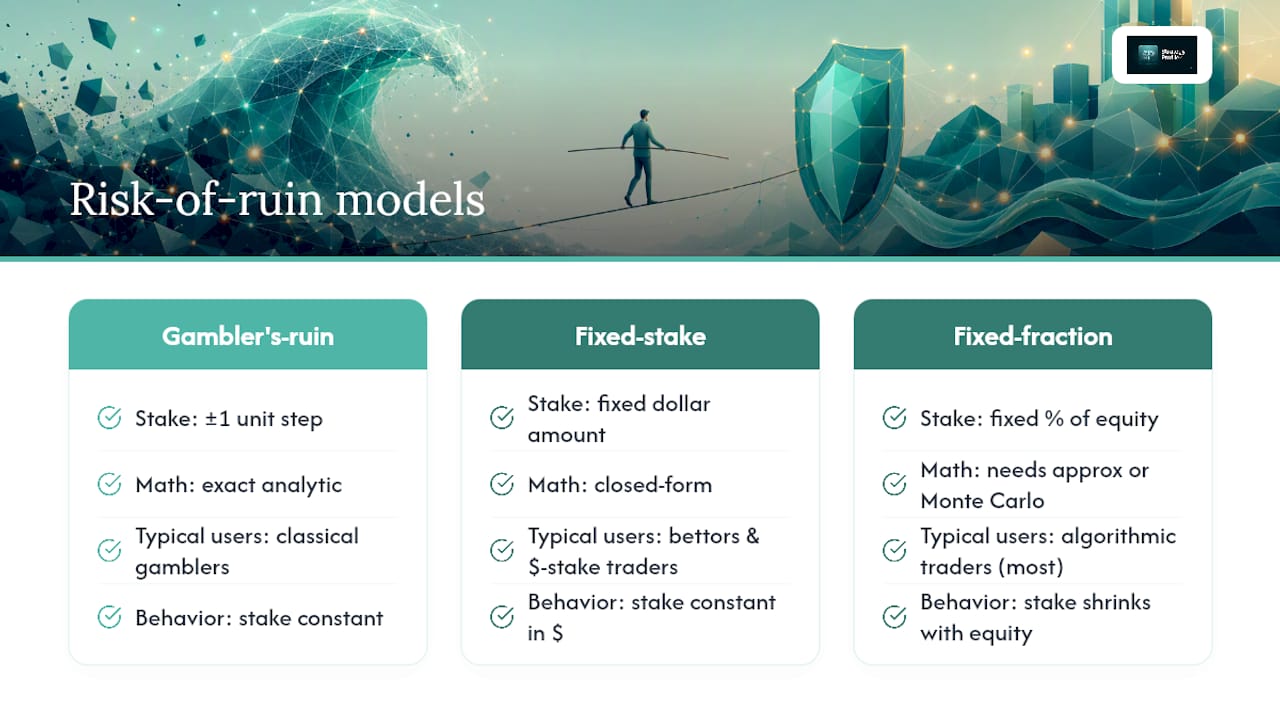
Three distinct flavors show up in practice.
Discrete gambler's-ruin treats each trade as a fixed ±1 unit step. You start with i units, the ruin threshold is zero, and the target is N units. The model is clean and mathematically exact, rooted in classical probability theory going back to Pascal and Huygens.
Fixed-stake betting generalizes this to real bet sizes: you risk a fixed dollar amount per trade rather than one abstract unit. The formulas stay closed-form but now depend on your actual bankroll, stake, win rate, and average odds.
Percentage-of-account (fixed-fraction) staking is what most algorithmic traders actually use. You risk a fixed percentage of current equity per trade, so the stake shrinks as the account shrinks. This compounding effect changes the math significantly and requires either an exponential approximation or Monte Carlo simulation.
Traders also choose between infinite-horizon models (what is the probability of ever hitting ruin?) and finite-horizon models (what is the probability of hitting ruin within the next 500 trades?). The infinite-horizon version is more conservative and more commonly cited. The finite-horizon version is more realistic for a trader with a defined season or funding cycle.
Common ruin thresholds in practice: full account wipeout (equity = 0), a defined drawdown percentage such as 50% of peak equity, or falling below the minimum margin required to hold positions. Prop firm traders often use the firm's maximum drawdown rule as their ruin threshold, which makes the calculation directly operational.
How to calculate risk of ruin: three methods
The discrete gambler's-ruin formula
For a game with fixed ±1 unit steps, win probability p, and loss probability q = 1 − p, starting with i units and targeting N units, the closed-form expressions are:
Biased game (p ≠ q):
P(ruin) = [1 − (p/q)^i] / [1 − (p/q)^N] × (q/p)^i ... simplified to:
P(success) = (1 − r^i) / (1 − r^N), where r = q/p
P(ruin) = 1 − P(success)
Fair game (p = q = 0.5):
P(success) = i / N, so P(ruin) = 1 − (i/N)
Expected duration for a fair game: D = i × (N − i) trades.
These formulas assume independent, identically distributed outcomes and a fixed stake every trade. They are exact within those assumptions, which is why they work well for screening and quick sanity checks.
Monte Carlo simulation
Monte Carlo is the right tool when your trade outcomes are not identically distributed, your stake size varies, you hold correlated positions, or your return distribution has fat tails. DayTradingToolkit recommends Monte Carlo as the most realistic estimate when returns are non-binary or stakes vary, and the guidance is to use your empirical trade distribution rather than a theoretical one.
For robust tail estimates, run enough simulations to stabilize the low-probability outcomes you care about. A few hundred simulations will give you a rough answer; a few thousand gives you a stable one.
Decision rule: use closed-form formulas for fast screening and initial sizing decisions. Switch to Monte Carlo when any of these apply: non-iid returns, variable stake sizing, fat tails, correlated positions across strategies, or a finite horizon with specific constraints like prop firm drawdown limits.
Pro Tip: Before interpreting any RoR output, verify your strategy has positive expected value. If EV ≤ 0, long-run ruin probability approaches 100% regardless of stake size. No formula can fix a negative edge.
A step-by-step calculator walkthrough
Inputs
| Input | Example value |
|---|---|
| Risk per trade | 2% ($200) |
| Win rate (p) | 0.55 |
| Reward-to-risk ratio | 1.5:1 |
| Ruin threshold | 50% drawdown ($5,000) |
| Trade horizon | 500 trades |
Step 1: Check expected value
Average win = $200 × 1.5 = $300. Average loss = $200.
EV per trade = (0.55 × $300) − (0.45 × $200) = $165 − $90 = +$75. Positive. Proceed.
Step 2: Discrete formula (fixed-stake approximation)
Using the GamblingCalc discrete model: with a starting bankroll of 50 units (at $200/unit), a ruin threshold of 25 units, win probability 0.55, and r = q/p = 0.45/0.55 ≈ 0.818:
P(success) = (1 − 0.818^50) / (1 − 0.818^75) ≈ very high, placing P(ruin) well below 1%.
Step 3: Diffusion approximation
Expectancy E ≈ +$75 per trade. Capital units to ruin U = 25 (the $5,000 gap divided by $200 stake). Variance σ² ≈ (0.55 × 300² + 0.45 × 200²) − 75² ≈ 49,500 + 18,000 − 5,625 = 61,875.
P(ruin) ≈ exp(−2 × 75 × 25 / 61,875) ≈ exp(−0.0606) ≈ 0.941, which means P(ruin) ≈ 6%.
That result looks alarming compared to the discrete formula. The difference is the model: the diffusion approximation accounts for the continuous compounding of losses, while the discrete model assumes fixed dollar stakes. The 6% figure is the more conservative and realistic estimate for a percentage-based trader.
Step 4: Validate and adjust
A 6% ruin probability exceeds the cautious threshold. Cut risk per trade to 1% ($100). Recalculate: U doubles to 50 units, E halves to roughly $37.50 per trade. P(ruin) ≈ exp(−2 × 37.5 × 50 / 15,469) ≈ exp(−0.242) ≈ 0.785, so P(ruin) ≈ 21%... wait. The variance also changes when stake changes. Recalculating σ² at $100 stake: ≈ 15,469. P(ruin) ≈ exp(−2 × 37.5 × 50 / 15,469) ≈ exp(−0.242) ≈ 22%. Still high because the ruin threshold in dollar terms also halved. Fix the ruin threshold at the original $5,000 (now 100 units at $100 stake): P(ruin) ≈ exp(−2 × 37.5 × 100 / 15,469) ≈ exp(−0.485) ≈ 38%... that's worse. The issue: halving the stake also halves expectancy in dollar terms, and the formula is sensitive to the ratio. This is exactly why you need to run the numbers, not guess.
Pro Tip: Run the diffusion approximation at multiple stake sizes and plot the curve. The nonlinear drop in ruin probability as you reduce stake size is the single most persuasive argument for conservative sizing.
How to read your RoR output and what the thresholds mean
A RoR percentage is not a timetable. It doesn't say "you will blow up in 300 trades." It says "given your current parameters, this is the probability of hitting your ruin threshold before your edge recovers you." That distinction matters because traders often treat a low RoR as a guarantee of survival. It isn't. A 5% RoR means roughly 1 in 20 traders running your exact system will hit ruin.
| RoR range | Risk profile | Practical meaning | Recommended action |
|---|---|---|---|
| < 1% | Conservative | Ruin is a remote tail event | Maintain sizing; monitor edge |
| 1–5% | Cautious | Meaningful but manageable risk | Review sizing; tighten drawdown rules |
| 5–6% | Aggressive | Elevated ruin risk over long horizons | Reduce position size immediately |
| > 5% | Dangerous | High probability of eventual wipeout | Stop trading; recalculate from scratch |
| EV ≤ 0 | Terminal | Long-run ruin is near-certain | Fix the strategy before sizing |
Professional guidance places the target for serious traders at sub-1% over their defined trade horizon. Retail traders often operate at 5–15% without realizing it, simply because they've never run the calculation.
Recovery math reinforces why the upper thresholds are so dangerous. A 50% drawdown requires a 100% gain to recover. A 75% drawdown requires a 300% gain. The asymmetry means that surviving to trade another day is worth more than any single trade's upside.
Risk of ruin vs. drawdown: why you need both numbers
Drawdown measures what already happened: the peak-to-trough decline in your account equity. Risk of ruin measures what might happen: the forward-looking probability of hitting a terminal threshold. They are related but not interchangeable, and conflating them is one of the most common mistakes in retail risk management.
Key distinctions:
- A strategy can show a large historical drawdown but carry a low RoR if per-trade risk is small and variance is bounded.
- A strategy can show a modest historical drawdown but carry a high RoR if the edge is thin and stake size is large relative to the bankroll.
- Drawdown is backward-looking and descriptive. RoR is forward-looking and probabilistic.
- A 30% historical drawdown tells you what happened in your backtest. A 3% RoR tells you the probability of a terminal loss in live trading.
Numeric illustration: two traders each have a 30% historical max drawdown. Trader A risk 0.5% per trade with a 60% win rate. Trader B risks 5% per trade with the same win rate. Their historical drawdowns look similar in a short backtest. Their RoR figures diverge dramatically, with Trader B facing a materially higher probability of ruin over a 1,000-trade horizon.
Investopedia's treatment of RoR in finance emphasizes this forward-looking character: the metric is specifically designed to capture the probability of catastrophic loss, not just describe past volatility.
When the formulas break down: assumptions and limitations
Closed-form RoR formulas rest on assumptions that real markets routinely violate. Knowing where the model fails is as important as knowing the formula.
Core assumptions:
- Trade outcomes are independent and identically distributed (i.i.d.)
- Edge and variance are constant across all trades
- Stake size is fixed (or fixed-fraction in the diffusion model)
- Positions are uncorrelated
- The horizon is either infinite or cleanly defined
Practical failure modes:
Fat tails. Real return distributions have more extreme outcomes than a normal distribution predicts. A single catastrophic loss can exceed what the formula treats as possible. The 2010 Flash Crash and the 2015 Swiss franc depegging are examples where tail events exceeded any reasonable variance estimate.
Regime shifts. A strategy's edge in a trending market may be negative in a ranging market. The formula assumes constant E, but live trading delivers changing E. When the regime shifts, your actual RoR is higher than the formula says.
Correlation spikes. During market stress, positions that appeared uncorrelated start moving together. Portfolio-level variance spikes exactly when you can least afford it.
Slippage and execution costs. These reduce realized expectancy below backtested expectancy, effectively shrinking E in the formula without the trader noticing.
Broker margin calls and position limits. These impose ruin thresholds the formula doesn't model, often triggering at worse prices than the theoretical threshold.
Decision checklist: use closed-form formulas when outcomes are roughly i.i.d., stakes are fixed or fixed-fraction, and positions are uncorrelated. Switch to Monte Carlo when any of those conditions fail, and use your empirical trade distribution rather than a theoretical one for the simulation inputs.
How institutional trading desks apply RoR
Professional desks treat survival as a binding constraint, not a metric to monitor. Position sizing is set to satisfy the RoR constraint first; return optimization comes second. That inversion is the single biggest difference between institutional and retail risk practice.
Typical desk workflow: define the trade horizon and ruin threshold upfront, compute per-strategy expectancy and variance from walk-forward validated backtests, calculate the marginal RoR contribution of each new position, and set aggregate position limits so that portfolio-level RoR stays within the target. Closed-form approximations handle the screening pass. Monte Carlo with realistic constraints handles the validation pass.
The University of Pittsburgh's academic derivations of gambler's-ruin probabilities show formally why even a small negative drift makes ruin nearly certain over long horizons, which is the mathematical foundation for why desks are so strict about edge verification before sizing.
Portfolio-level checklist for algorithmic traders:
- Define your ruin threshold (absolute drawdown, percentage, or prop firm rule).
- Define your trade horizon (number of trades or calendar period).
- Estimate per-strategy expectancy and variance from validated backtests.
- Compute RoR for each strategy individually using the diffusion approximation.
- Estimate portfolio-level variance accounting for inter-strategy correlation.
- Compute aggregate portfolio RoR and compare to your target.
- Adjust position sizes until portfolio RoR meets the target.
- Set a monitoring cadence: recalculate after every 50–100 live trades to detect edge degradation.
Pro Tip: Adopt a survival-first sizing rule: never increase position size until live trading confirms the edge you estimated in backtesting. The cost of starting small is a few weeks of lower returns. The cost of starting large with an overestimated edge can be the account.
How bet size volatility affects your ruin probability
Variable stake sizing is one of the most underappreciated sources of elevated RoR. The closed-form formulas assume a fixed stake. When your actual trade sizes fluctuate, whether because you're scaling in, adjusting for volatility, or simply being inconsistent, the effective variance of your returns increases even if your average stake stays the same.
Higher variance directly increases RoR in the diffusion formula: σ² is in the denominator of the exponent, so larger variance produces a smaller (less negative) exponent and a higher ruin probability. A trader who sometimes risks 1% and sometimes risks 4% does not have the same RoR as a trader who consistently risks 2.5%, even though the average is identical. The inconsistent trader faces higher ruin risk because the large-stake trades create outsized loss events.
This has a practical implication: consistency in position sizing is itself a risk management tool. Erratic sizing, even when the average looks acceptable, degrades your survival odds in ways the simple formula won't capture unless you model the actual stake distribution. Monte Carlo handles this correctly; closed-form does not.
Risk of drawdown alongside risk of ruin: a complete picture
Risk of drawdown asks a different question than risk of ruin: what is the probability of experiencing a drawdown of at least X% at some point during your trading horizon? It's a softer threshold than ruin, and it's the metric that matters most for psychological and operational sustainability.
The calculation follows similar logic to RoR. For a fixed-fraction system, the probability of experiencing a drawdown of depth D before recovering can be approximated using the same exponential framework, substituting D as the threshold rather than full ruin. The result is always higher than the ruin probability for the same horizon, because a drawdown of 30% is easier to hit than full ruin.
Why track both? Risk of ruin tells you whether your strategy can survive. Risk of drawdown tells you whether you can survive your strategy. A trader who mathematically has a 0.5% ruin probability but a 60% probability of a 40% drawdown may abandon the strategy during that drawdown, effectively self-imposing ruin. The behavioral dimension is real and the math supports it: size conservatively enough that the probable drawdown range stays within your psychological tolerance, not just within your mathematical survival zone.
Historical cases where risk of ruin played out
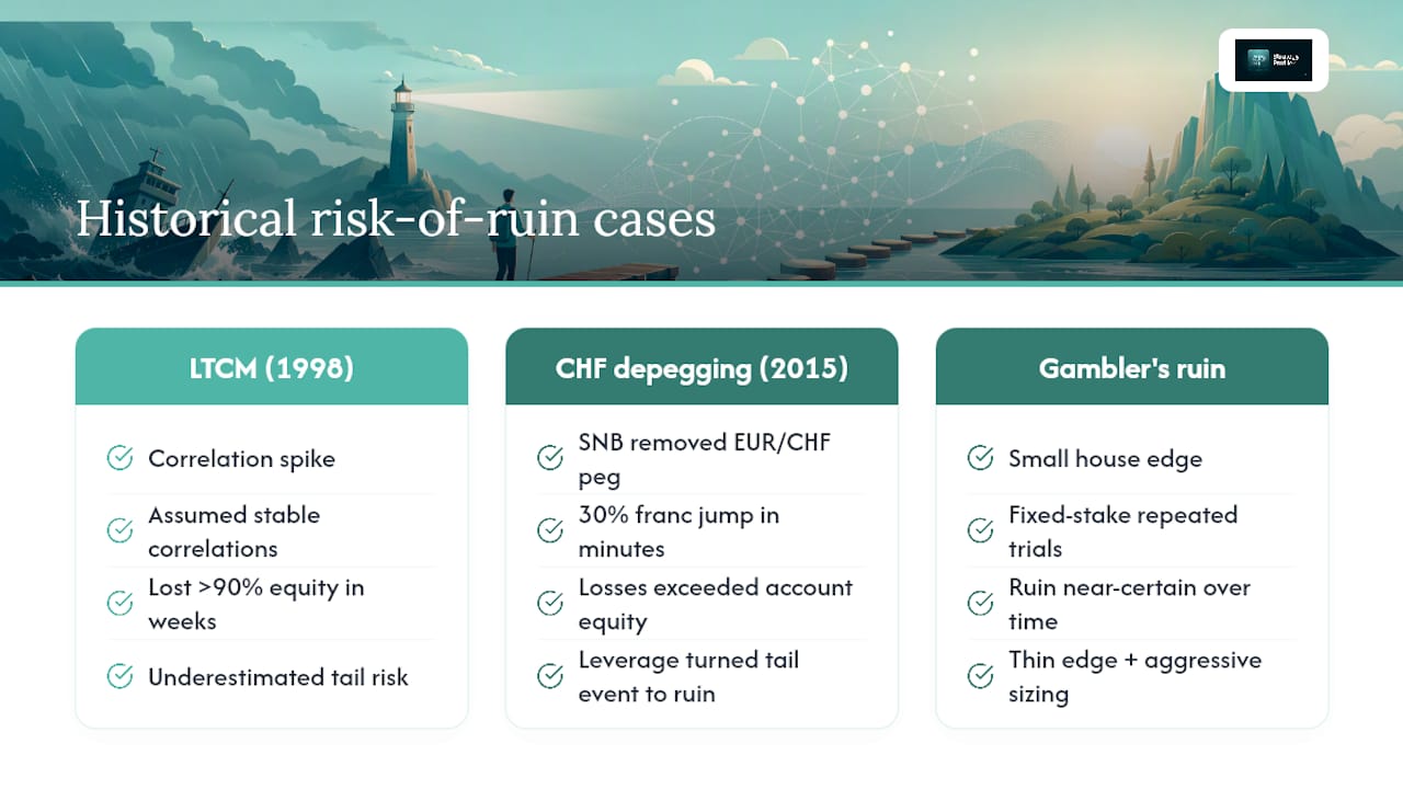
Long-Term Capital Management (1998). LTCM was run by some of the most sophisticated quantitative traders in the world, including Nobel laureates. Their models showed near-zero ruin probability under normal market conditions. What the models didn't account for was the correlation spike during the Russian debt crisis: positions that were modeled as uncorrelated moved together catastrophically. Portfolio-level variance exploded beyond any historical estimate. The fund lost over 90% of its equity in weeks. The failure was not a bad strategy. It was a model that assumed stable correlations and underestimated tail risk.
The 2015 Swiss franc depegging. The Swiss National Bank's sudden removal of the EUR/CHF floor on January 15, 2015 moved the franc roughly 30% in minutes. Traders and brokers holding leveraged positions faced losses that exceeded their entire account equity, a scenario where the ruin threshold was hit before a stop-loss could execute. Fixed-stake RoR formulas assigned near-zero probability to a 30% single-candle move. The actual probability was low but not zero, and leverage turned a tail event into an account-ending event for many retail traders.
The gambler's ruin in practice. The Wikipedia treatment of risk of ruin and the University of Pittsburgh's probability derivations both show that even a small house edge, applied over enough trials, makes ruin near-certain for a fixed-stake player. Casino operators have known this for centuries. The lesson for traders is identical: a thin or uncertain edge, combined with aggressive sizing, produces ruin on a long enough timeline regardless of short-term results.
Key Takeaways
Risk of ruin is the single most important survival metric for any trader: a positive edge means nothing if your position sizing guarantees you'll blow up before the edge pays out.
| Point | Details |
|---|---|
| RoR definition | Probability your account hits a ruin threshold before your edge recovers it. |
| Most powerful lever | Reducing risk per trade lowers RoR nonlinearly; cutting from 3% to 1% can dramatically improve survival odds. |
| Acceptable thresholds | Conservative traders target below 1%; above 5% requires immediate position size reduction. |
| When to use Monte Carlo | Use simulation when stakes vary, positions correlate, or returns show fat tails. |
| Strategyprofilers | Combines multiple EA equity curves, runs walk-forward validation, and optimizes lot sizes against drawdown and RoR targets at the portfolio level. |
The math is only half the problem
Most traders who study RoR come away focused on the formula. That's the wrong takeaway. The formula is a planning tool. The real problem is behavioral: traders who calculate a safe stake size in calm conditions increase it after a winning streak, reduce it after a loss (often at the worst moment), and abandon the system during the inevitable drawdown that the math already predicted.
The survival-first approach that institutional desks use isn't just about the numbers. It's about treating the RoR constraint as non-negotiable regardless of recent performance. A 0.5–1% risk-per-trade starting point isn't conservative because the math demands it. It's conservative because it keeps the probable drawdown range within a zone where most traders can stay rational and stay in the trade.
Combine the math with operational limits: a daily max loss rule, a hard stop on adding positions during drawdowns, and a regular recalculation cadence. The formula tells you the probability. The operational rules are what make you act on it.
Strategyprofilers brings portfolio-level RoR analysis to algorithmic traders
Calculating RoR for a single strategy is straightforward. Doing it across a portfolio of Expert Advisors, where strategies interact, correlate, and share capital, is where most traders hit a wall.
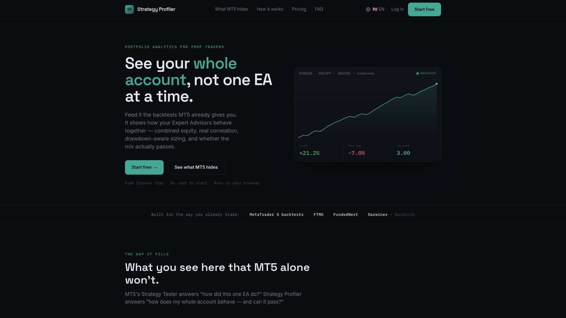
Strategyprofilers addresses exactly that problem. The platform combines multiple EA equity curves into a single portfolio view, runs walk-forward validation and bootstrap confidence intervals to test whether your backtested edge is real, and optimizes lot sizes against specific drawdown and performance targets. For prop firm traders, it includes compliance testing against firm-specific drawdown rules, which means your ruin threshold is built directly into the sizing calculation. The result is a portfolio-level RoR picture that a single-strategy calculator simply can't give you. Start your analysis and find out whether your current sizing survives the math.
Useful sources
-
Gambler's Ruin (University of Pittsburgh, J. D. Norton) — Academic derivations of gambler's-ruin probabilities with worked examples. Best for understanding the theoretical foundations and why small negative drift makes ruin near-certain.
-
Risk of Ruin (Wikipedia) — Concise summary of discrete and random-walk models with closed-form expressions for fair and biased games. Good starting reference for formula verification.
-
Gambler's Ruin Calculator, Discrete Model (GamblingCalc) — Interactive discrete-model calculator for biased and fair games. Use for quick fixed-stake RoR estimates and expected duration calculations.
-
Risk of Ruin Calculator (GamblingCalc) — Practical calculator covering bankroll, unit size, win rate, and average odds. Includes break-even win rate output and explicit cautions about fixed-stake model limits.
-
Risk of Ruin, Trader Edition (SatoshiMacro) — Implements the exponential approximation P(ruin) is approximately calculated by an exponential formula involving expectancy, capital units, and variance, indicating that increasing expectancy or capital units, or decreasing variance, reduces ruin probability exponentially. with trader-focused inputs. Best for fixed-fraction sizing calculations.
-
Risk of Ruin in Trading (DayTradingToolkit) — Practical guide connecting RoR to position sizing and recovery math. Recommends Monte Carlo for non-binary return distributions.
-
What Is Risk of Ruin? (The Planet Indicator) — Rule-of-thumb guidance on the 1–2% risk-per-trade threshold and when to escalate to simulation.
-
Risk of Ruin: What It Means (Investopedia) — Broad finance and trading definition with notes on VaR, Monte Carlo modeling, and diversification strategies.