

Trading expectancy is the average profit or loss you should expect per trade. One number. One test. If it's positive, your strategy has an edge. If it's negative, no amount of discipline or position sizing saves it.
The formula exists in two forms, and you'll want both:
- Dollar form: Expectancy = (Win% × Avg win) − (Loss% × Avg loss)
- R-multiple form: Expectancy = (Win% × Avg win in R) − (Loss% × Avg loss in R)
A positive result means the strategy earns money over a large sample. A negative result means it bleeds, regardless of how good any individual week looks. Profit Factor and R-multiples give you complementary angles on the same question, and tools like Strategyprofilers let you run this analysis across an entire portfolio of Expert Advisors rather than one setup at a time.
The hard truth: Research from Berkeley shows that persistent net profitability in day trading is rare. The traders who survive long-term are the ones who measure skill after fees, not before.
Table of Contents
- What is trading expectancy and how do you calculate it?
- Step-by-step worked example: dollars and R-multiples
- What counts as a good expectancy? R-multiple benchmarks
- How many trades do you need before trusting your expectancy?
- Common pitfalls that make expectancy misleading
- Four levers for improving your expectancy
- How R-multiples and position sizing connect to account growth
- Applying expectancy across a portfolio of strategies
- How expectancy relates to win rate, profit factor, and drawdown
- How does expectancy relate to risk-adjusted returns like the Sharpe ratio?
- Using Monte Carlo simulations to project long-term outcomes
- How expectancy integrates with money management frameworks
- Common misconceptions about expectancy
- Key Takeaways
- The metric most traders underuse
- Strategyprofilers turns expectancy analysis into a portfolio-level system
- Useful sources
What is trading expectancy and how do you calculate it?
Expectancy combines two things most traders track separately: how often they win, and how much they win or lose when they do. Neither metric alone tells you whether a strategy is profitable. A 70% win rate with tiny winners and large losers produces negative expectancy. A 35% win rate with a 3:1 reward-to-risk ratio produces positive expectancy. The formula synthesizes both into a single diagnostic.
The components:
- Win%: Number of winning trades ÷ total trades
- Loss%: 1 − Win% (or losing trades ÷ total trades)
- Avg win: Mean dollar profit across all winning trades
- Avg loss: Mean dollar loss across all losing trades (expressed as a positive number)
Why R-multiples matter. R is the amount risked on a single trade, defined by your stop loss. Expressing wins and losses as multiples of R strips out position-sizing distortions and lets you compare expectancy across strategies with different account sizes or lot sizes. A strategy with 0.3R expectancy is directly comparable to another with 0.1R expectancy, regardless of whether one trades $500 lots and the other trades $50,000 lots.
What counts as net P&L. Gross expectancy routinely overstates live performance once commissions, spreads, slippage, and borrow fees are deducted. Always compute expectancy on net P&L. Reconcile your trade journal against your broker statement before running the numbers.
Pro Tip: Build your trade log with a column for gross P&L and a separate column for net P&L after all costs. Run the expectancy formula on the net column only. Gross expectancy is a vanity metric.
Step-by-step worked example: dollars and R-multiples
Here's a 15-trade sample log. Work through it once in dollars, then convert to R.
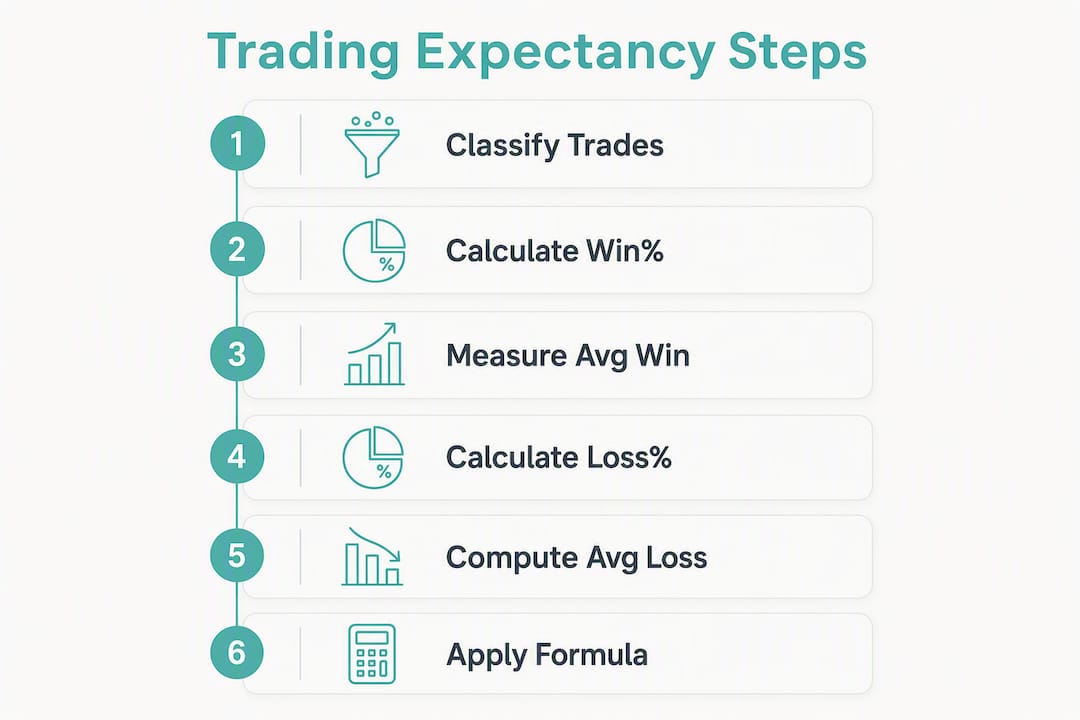
Step 1: Classify and total the trades.
| Trade | Result | Gross P&L | Costs | Net P&L | R risked | Net R |
|---|---|---|---|---|---|---|
| 1 | Win | — | $8 | — | $100 | — |
| 2 | Loss | — | $8 | — | $100 | — |
| 3 | Win | — | $8 | — | $100 | — |
| 4 | Loss | — | $8 | — | $100 | — |
| 5 | Win | — | $8 | — | $100 | — |
| — | Loss | — | $8 | — | $100 | — |
| 7 | Win | — | $8 | — | $100 | — |
| 8 | Loss | — | $8 | — | $100 | −1.03 |
| 9 | Win | $230 | $8 | $222 | $100 | +2.22 |
| 10 | Loss | — | $8 | −$118 | $100 | −1.18 |
| 11 | Win | $190 | $8 | $182 | $100 | +1.82 |
| 12 | Loss | −$100 | $8 | −$108 | $100 | −1.08 |
| 13 | Win | $260 | $8 | $252 | $100 | +2.52 |
| 14 | Loss | −$92 | $8 | −$100 | $100 | −1.00 |
| 15 | Win | $200 | $8 | $192 | $100 | +1.92 |
Step 2: Compute the inputs.
- Wins: 8 trades. Losses: 7 trades. Win% = 8/15 (a little more than half). Loss% = a little less than half.
- Avg net win (dollars) is the mean of the winning trade profits.
- Avg net loss (dollars) is the mean of the losing trade losses.
Step 3: Run the formula.
Dollar expectancy calculation shows a positive expected profit per trade.

R-multiple expectancy calculation shows a positive expected return of about +0.7R per trade.
Step 4: Interpret. Positive expectancy at +0.70R is strong. The strategy earns roughly 70 cents per dollar risked, on average, across this sample.
Common mistakes to avoid:
- Mixing gross P&L for wins with net P&L for losses (or vice versa)
- Using different R definitions across trades (e.g., sometimes using account % and sometimes using dollar stop)
- Running the formula on fewer than 30 trades and treating the result as reliable
Pro Tip: Paste this table structure into Google Sheets or Excel. Add a row for each new trade. The formula cells update automatically, giving you a live expectancy dashboard.
What counts as a good expectancy? R-multiple benchmarks
R-multiple thresholds give you a practical grading scale:
- Above 0.5R: Excellent. Rare in live trading, and worth scrutinizing for overfitting before scaling.
- 0.3R–0.5R: Solid and reliable. Most professional systematic strategies sit here.
- 0.1R–0.3R: Marginal. The strategy works, but execution costs and slippage eat into it fast. High-frequency setups can survive here; low-frequency ones often can't.
- At or below 0R: The strategy fails to cover operating costs. No position sizing trick fixes this.
Context matters as much as the number itself. A scalping strategy executing 200 trades per month at 0.15R expectancy generates more expected return than a swing strategy at 0.4R executing 10 trades per month, purely because of frequency. Consistent traders typically maintain a Profit Factor between 1.3 and 1.8; values above 3 often signal curve-fitting rather than genuine edge.
Watch the cost sensitivity. A strategy sitting at 0.15R expectancy on gross P&L can flip to −0.05R after a $5 commission increase per trade. Marginal strategies have almost no buffer.
How many trades do you need before trusting your expectancy?
Treat anything under 30 trades as anecdote, 30–100 as a rough sketch, and 100+ as data worth acting on for a given setup. That's the practitioner standard, and it's conservative for a reason.
Expectancy stabilizes slowly because it's a mean of a distribution that can have fat tails. A single outlier trade, a 5R winner or a 3R loss, can shift your observed expectancy by 0.1R or more on a 30-trade sample. On a 200-trade sample, the same outlier barely moves the needle.
Practical checks for stability:
- Rolling expectancy: Plot expectancy over the last 20 or 50 trades on a rolling basis. A stable edge produces a line that oscillates around a consistent value. A deteriorating edge trends downward.
- Split-sample testing: Divide your trade history in half chronologically. If expectancy is materially different between the two halves, the edge may be regime-dependent.
- Walk-forward and bootstrap checks: Run the strategy on out-of-sample data or use bootstrap resampling to estimate confidence intervals around your expectancy estimate.
Low-frequency setups face a compounding problem: a strategy that trades 15 times per month needs nearly seven months to accumulate 100 trades. Monitoring expectancy stability across market regimes is especially important here, because the market can shift before you have enough data to detect it.
Pro Tip: Use walk-forward validation and bootstrap confidence intervals to estimate how wide the band around your expectancy estimate actually is. A result of +0.3R ± 0.4R is not a reliable edge. A result of +0.3R ± 0.08R is.
Common pitfalls that make expectancy misleading
Most expectancy calculations in the wild are wrong. Not slightly off. Wrong in ways that flip the sign.
- Gross instead of net P&L: The most common error. Commissions, spreads, and slippage are not optional deductions. They're the cost of doing business, and they belong in the denominator.
- Slippage on stops: If your backtester assumes perfect fill at your stop price and live trading fills 2–3 pips worse, your average loss is understated in every backtest.
- Survivorship and selection bias: Backtesting only on instruments or periods that survived, or cherry-picking the date range where the strategy happened to work, inflates expectancy. The strategy never saw the regimes that would have hurt it.
- Overfitting: A strategy optimized on in-sample data to maximize expectancy will almost always show lower expectancy on out-of-sample data. The gap between the two is the overfitting tax.
Corrective actions are straightforward: compute expectancy on net P&L only, enforce out-of-sample testing before trusting any backtest result, require a minimum of 100 trades per setup, and log slippage per trade so you can reconcile gross versus net systematically.
Academic research confirms that persistent net profitability is rare precisely because most traders don't account for these costs rigorously. The ones who do are the ones whose expectancy estimates hold up in live trading.
Four levers for improving your expectancy
Expectancy has exactly four inputs you can move: win rate, average win, average loss, and trade frequency. Improving any one of them without degrading the others raises expectancy.
- Raise win rate without shrinking winners. Add confirmation filters that eliminate low-probability setups. If a filter removes 20% of your trades but those trades were mostly losers, win rate rises without touching average win size.
- Grow average win. Let profitable trades run longer before exiting. Trailing stops and scaled exits both help. The risk is that holding longer sometimes turns winners into losers, so measure the net effect on expectancy, not just on the biggest wins.
- Shrink average loss. Honor your stops. Every time you move a stop wider "just this once," you're inflating average loss. Tighter execution discipline, not tighter stops, is the fix.
- Increase frequency of genuine edges. More trades at positive expectancy compounds faster. But adding frequency by lowering your setup criteria usually degrades win rate and average win simultaneously. Only add frequency when the new setups pass the same expectancy threshold as your existing ones.
The see-saw tradeoff is real: raising win rate often requires tighter reward-to-risk ratios, which shrinks average win. Measure every change by its effect on the full expectancy formula, not by any single component. Win rate alone is a deceptive metric because it ignores the magnitude of what you win or lose.
Pro Tip: Run an A/B test on your setup filters. Apply the new filter to the second half of your historical data only, compute expectancy for both halves, and compare. If the filtered version shows higher expectancy on data it never saw during development, the filter is probably adding real signal.
How R-multiples and position sizing connect to account growth
Expectancy expressed in R is the cleanest input for sizing math. Here's why: once you know your per-trade expectancy in R and your trade frequency, you can project expected annual return in R-multiples directly.

Expected annual return (in R) = Expectancy per trade × Trades per year
A strategy with 0.3R expectancy executing 150 trades per year produces an expected return of 45R annually. If you risk 1% of account per trade, that's approximately 45% expected annual return before compounding effects. At 0.5% risk per trade, it's roughly 22.5%.
Key considerations for sizing:
- Kelly criterion gives the theoretically optimal fraction to risk per trade. For a strategy with 0.3R expectancy and a 1:1 average win/loss ratio, full Kelly suggests a large risk fraction. In practice, traders use fractional Kelly (typically 25–50% of full Kelly) to reduce variance and drawdown.
- Fractional Kelly sacrifices some expected growth for much lower volatility. Most systematic traders find that full Kelly produces drawdowns they can't stomach psychologically or operationally.
- Monte Carlo projections use your net expectancy and its variance to simulate thousands of possible equity paths. The spread of those paths shows you realistic best-case and worst-case outcomes, not just the expected value.
A small positive expectancy of +0.2R–+0.3R compounds into material yearly returns given sufficient frequency and consistent sizing. The edge doesn't have to be large. It has to be real and consistent.
Applying expectancy across a portfolio of strategies
Single-strategy expectancy is the starting point. Portfolio-level expectancy is where algorithmic traders actually operate.
When you run multiple Expert Advisors simultaneously, their individual expectancies don't simply add up. Correlation matters. Two strategies with 0.3R expectancy that are highly correlated produce roughly the same drawdown profile as one strategy. Two strategies with 0.3R expectancy that are negatively correlated produce a smoother combined equity curve with lower peak drawdown.
Portfolio-level questions expectancy analysis must answer:
- How do the individual strategies' expectancies combine into a portfolio-level edge?
- Where is risk concentrated, and which EAs are effectively duplicating each other's exposure?
- What lot sizing across the portfolio meets a specific drawdown target?
Walk-forward validation and bootstrap confidence intervals answer a different question: not "what was the expectancy?" but "how stable is it, and what's the realistic range?" A strategy showing +0.4R expectancy in-sample with a bootstrap confidence interval of ±0.35R is not a reliable foundation for live allocation.
| Portfolio analysis feature | What it tells you |
|---|---|
| Combined equity curve | Aggregate P&L and drawdown across all EAs simultaneously |
| Correlation matrix | Which EAs are effectively duplicating exposure |
| Portfolio lot-size optimizer | Allocation that meets a specific drawdown or return target |
| Walk-forward validation | Whether in-sample expectancy holds on out-of-sample data |
| Bootstrap confidence intervals | Realistic range around your expectancy estimate |
Pro Tip: Monitor rolling expectancy per strategy on a 30-trade window. When a strategy's rolling expectancy drops below zero for two consecutive windows, reduce its allocation before the drawdown compounds. Don't wait for the equity curve to tell you what the expectancy already showed.
How expectancy relates to win rate, profit factor, and drawdown
These three metrics are not alternatives to expectancy. They're complements that answer different questions.
Win rate tells you how often you're right. It says nothing about whether being right is worth anything. A 90% win rate with a 10:1 loss-to-win ratio produces negative expectancy. Expectancy synthesizes both frequency and magnitude into the single number that actually matters for profitability.
Profit Factor is gross profit divided by gross loss. A Profit Factor of 1.5 means the strategy earns $1.50 for every $1.00 lost. It's a useful robustness signal: consistent traders often maintain Profit Factor between 1.3 and 1.8, while values above 3 frequently indicate overfitting. Profit Factor doesn't tell you how fast the account grows; expectancy does.
Drawdown is the sizing risk. A strategy with strong expectancy but high variance in trade outcomes can produce severe drawdowns at standard risk levels. Expectancy tells you the direction of travel; drawdown tells you how rough the road is. Pair them: a strategy with +0.3R expectancy and a 25% maximum drawdown at 1% risk per trade is a very different proposition than one with the same expectancy and a 10% maximum drawdown.
How does expectancy relate to risk-adjusted returns like the Sharpe ratio?
Expectancy measures edge per trade. The Sharpe ratio measures return per unit of volatility over time. They're related but not interchangeable.
A strategy with high expectancy but wildly variable trade outcomes (some trades at +5R, most at −1R) can produce a low Sharpe ratio because the volatility of returns is high relative to the mean. A strategy with modest expectancy and very consistent trade outcomes produces a higher Sharpe ratio. For position sizing and capital allocation decisions, the Sharpe ratio is often more useful than raw expectancy because it accounts for the bumpiness of the equity curve, not just its direction.
The practical link: net R-based expectancy is the numerator of a trade-level Sharpe calculation. Divide your average net R per trade by the standard deviation of your per-trade R outcomes, then scale by the square root of annual trade frequency. That gives you an annualized Sharpe estimate directly from your trade log, without needing daily equity curve data.
Using Monte Carlo simulations to project long-term outcomes
Monte Carlo simulation takes your observed expectancy and its variance and runs thousands of randomized sequences of trades. Each sequence produces a different equity path. The distribution of those paths shows you the realistic range of outcomes, not just the expected value.
Why this matters: a strategy with +0.3R expectancy and high variance might show a 15% probability of a 40% drawdown within 200 trades even though the expected outcome is positive. That's information you need before sizing up.
The inputs are your net expectancy, the standard deviation of per-trade R outcomes, and your trade frequency. Most simulation tools let you specify starting capital and risk per trade, then output percentile equity curves (10th, 50th, 90th percentile paths). The gap between the 10th and 90th percentile paths is a direct function of variance, which is why low-variance strategies with modest expectancy often produce tighter, more predictable outcome distributions than high-variance strategies with higher expectancy.
How expectancy integrates with money management frameworks
Expectancy is the prerequisite for any money management framework. Fixed fractional sizing, Kelly criterion, and optimal f all require a positive expectancy as their starting condition. Apply them to a negative-expectancy strategy and they optimize the rate of loss, not the rate of growth.
Fixed fractional sizing (risking a fixed percentage of account per trade) is the most common framework. The percentage you choose determines both your expected growth rate and your expected drawdown. At 1% risk per trade with 0.3R expectancy, your expected gain per trade is 0.3% of account. At 2% risk, it's 0.—%, but your drawdown in a losing streak doubles.
The Kelly criterion maximizes long-run geometric growth but produces drawdowns most traders find unacceptable. Fractional Kelly (25–50% of the Kelly fraction) is the practical standard. The key input is net expectancy in R, which is why computing it accurately matters so much before touching position sizing at all.
Common misconceptions about expectancy
"High win rate means positive expectancy." It doesn't. A 75% win rate with average wins of $50 and average losses of $200 produces expectancy of (0.75 × $50) − (0.25 × $200) = $37.50 − $50 = −$12.50. Negative.
"Positive expectancy guarantees profit in the short run." It doesn't. Expectancy is a long-run average. In any short sequence of trades, variance dominates. A strategy with +0.3R expectancy can lose money for 30 consecutive trades. That's not a sign the edge is gone; it's normal variance.
"Expectancy is stable once calculated." Expectancy shifts across market regimes. A strategy that shows +0.4R in trending markets may show −0.1R in ranging markets. Treating a historical expectancy estimate as permanent is one of the most expensive mistakes in systematic trading.
"Gross expectancy is good enough." It isn't. The difference between gross and net expectancy is the difference between a strategy that looks profitable in a backtest and one that actually is profitable in live trading.
Key Takeaways
Trading expectancy, calculated as (Win% × Avg win) − (Loss% × Avg loss) on net P&L, is the single number that determines whether a strategy has a real edge, and R-multiples make that number portable across strategies and account sizes.
| Point | Details |
|---|---|
| Always use net P&L | Compute expectancy after commissions, spreads, and slippage — gross figures routinely overstate live performance. |
| R-multiple benchmarks | Above 0.5R is excellent; 0.3R–0.5R is solid and reliable; 0.1R–0.3R is marginal and vulnerable to execution costs; at or below 0R means the strategy cannot cover operating costs. |
| Sample size discipline | Fewer than 30 trades is anecdote; 100+ trades per setup is the minimum for reliable expectancy estimates. |
| Small edges compound | A +0.2R–+0.3R expectancy produces material annual returns with consistent sizing and sufficient trade frequency. |
| Strategyprofilers for portfolio-level work | Strategyprofilers combines equity curves, correlation analysis, walk-forward validation, and bootstrap confidence intervals to operationalize expectancy across multiple EAs simultaneously. |
The metric most traders underuse
Most traders check expectancy once, after a backtest, then move on. That's the wrong workflow. Expectancy is most useful as a live monitoring metric, not a one-time calculation.
Rolling expectancy on a 20 or 30-trade window tells you whether the edge is holding in current market conditions before the drawdown becomes obvious on the equity curve. A strategy that was delivering +0.35R six months ago and is now delivering +0.05R on a rolling basis hasn't failed yet, but it's telling you something. The question is whether you're listening.
The behavioral shift expectancy encourages is underrated. When you measure your trading system rather than individual trades, losses stop feeling like failures and start feeling like budgeted costs. A losing trade on a positive-expectancy strategy is not a mistake. A winning trade on a negative-expectancy strategy is not evidence of skill. That reframe alone changes how most traders respond to drawdowns.
Operationally, keep trade-level metadata: entry time, order type, slippage per trade, and gross versus net P&L. Without that data, you can't reconcile why your live expectancy differs from your backtest expectancy. And it will differ. The question is by how much, and whether the difference is explainable.
Strategyprofilers turns expectancy analysis into a portfolio-level system
Calculating expectancy for one strategy is a spreadsheet problem. Calculating it across a portfolio of Expert Advisors, monitoring it in real time, and sizing positions to meet specific drawdown targets is a different challenge entirely.
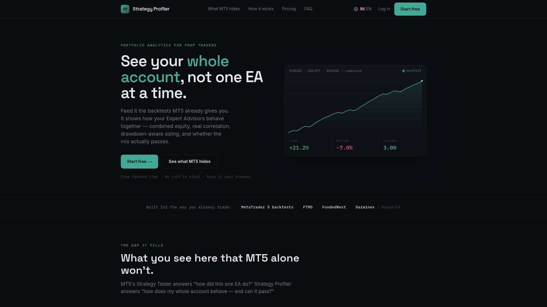
Strategyprofilers is built for exactly that. The platform generates combined equity curves across multiple EAs, runs correlation analysis to flag over-concentration, and optimizes lot sizing against custom performance and drawdown targets. Walk-forward validation and bootstrap confidence intervals give you a realistic range around your expectancy estimates, not just a point estimate that looks good in-sample. Real-account tracking lets you compare live results against backtest expectations trade by trade, so you catch regime shifts before they compound.
If you're running more than one EA or evaluating strategies for a prop firm challenge, the difference between a spreadsheet and a dedicated portfolio analytics platform shows up fast. Start with Strategyprofilers to see how your strategies' expectancies combine, where your risk is concentrated, and whether your current sizing matches your actual edge.
Useful sources
Primary research and further reading used in this guide:
- The Cross-Section of Speculator Skill — Berkeley faculty paper on persistent net profitability among day traders; foundational for understanding why net expectancy matters more than gross.
- Trading Expectancy Explained: How to Know If Your Edge Actually Works — Practitioner-friendly definition and formula walkthrough; good starting point for the calculation.
- Win Rate vs. Expectancy — Worked examples showing how win rate misleads and why expectancy synthesizes both frequency and magnitude; includes sample-size guidance.
- What Is Profit Factor in Trading? — Covers Profit Factor benchmarks (1.3–1.8 for consistent traders) and the relationship between Profit Factor and expectancy; includes the net P&L reconciliation warning.
- Trading Statistics and Data — Real trader performance data and guidance on monitoring expectancy stability across market regimes.
- Expectancy Formula — R-multiple thresholds and interpretation; useful reference for the benchmarks section.
- Informed Trading and Expected Returns (NBER) — Academic context on information asymmetry and cross-sectional return differences; relevant background for understanding persistent edge.